The simplest mathematical description of Ro: Infectious contacts β per unit time, all assumed infected, and disease with infectious (latent incubation) period of 1/γ, (frequency), then the basic reproduction number is R0 = β/γ. Diseases have multiple latency periods; therefore, the reproduction number for the disease is the sum of reproduction numbers for each transition time (Rt). The effective reproduction number, Re, changes with time, affected populations, and circumstances. The reproduction number, as widely used and referred to, appropriately and inappropriately, hides that transmission is stochastic not deterministic, often dominated by a small number of individuals, and heavily influenced by superspreading events https://journals.plos.org/plosbiology/article?id=10.1371/journal.pbio.3000897. The complexities of tracking, and therefore, mitigating infectious diseases, when they get out of hand, like COVID, limit the usefulness and predictability of mathematical models. Coronaviruses, as a group and SARS-CoV-2 in particular, confound Ro values; they can be easily blocked by barriers (masks, etc), distance, quarantine, and other environmental factors but are highly efficient in infecting hosts exposed to an infectious dose; this keeps overall % of infection low, but sustains virus in the population indefinitely. All this calculating gives one the sense of potentially great precision and accuracy in detecting an infectious disease in the environment, in reservoir or primary hosts, whether the infection is apparent or not, if one only has a test that is sensitive enough, has a low false positive rate, and one collects enough samples. In practice, many infectious agents, including SARS-CoV-2, are not so homogeneously distributed or even distributed normally. They favor certain niches and circumstances. Most of what one collects are samples of “empty space, volume” in respect to the agent, where the probability of detecting it in spite of the size of the sampled volume is zero. This condition is what defeats the models and mathematics. The math and models can be beautiful and sophisticated and the calculations perfect but “garbage in, garbage out” or “empty space in, empty space out!”Testing must give the idea of prevalence of active cases, recovered resistant individuals, and their respective density distribution in a population to have any idea of the probability of effective or failed transmission or growth rate of a local epidemic or global pandemic. The Ro (Re, more realtime) value is not very valuable for predicting absolute numbers of a population which will be infected but better for predicting how to stop an epidemic or pandemic, and it is not trivial to accurately calculate https://royalsociety.org/-/media/policy/projects/set-c/set-covid-19-R-estimates.pdf. So in the simplest terms what does the Ro value tells us, especially since it continuously changes into different Rt and Re subsets? Does it tell us, without resorting to history, what conditions have to be met over time? When a disease will move from endemic to epidemic? Ideally, the answer is yes to the second question, and how it is done, the answer to the first question, theoretically, has been made quite simple and clear, as math is supposed to do after, what seems to those of us who are not mathematicians, very much a confusing and esoteric series of symbolic manipulations and calculations. To put the answer most succinctly, R0, R naught, the basic reproduction number, the average number of other people each infected person must infect in a population, who are susceptible to the disease, in order to maintain the disease endemically (without any outside introduction or change which influences the number of infected to grow) or for it to go epidemic (exponentially in number of infected people or animals), or eventually pandemic (super exponential because of the interaction in space and time of many populations). For the endemic case:
For an infectious disease to die out after introduction:
For an infectious disease to become epidemic:
For it to become pandemic:
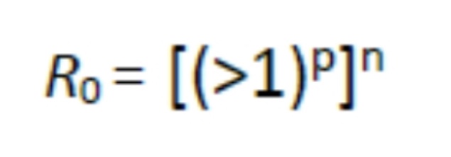
Where n is the number of separate susceptible populations which may be connected by the infectious agent being transported from one susceptible population to another through space and p is the exponential multiplication of the original source contacts which will become sources for spread to new populations. For an infectious disease to remain in the endemic state, the basic reproduction number and the proportion of the population susceptible must be inversely related, otherwise it will disappear or become epidemic and, perhaps, pandemic. This all assumes the susceptible hosts subject to exposure are exposed under the same circumstances with the highest probability of infection. Here is where the simple math gets complicated and I will not pursue it here but will just say it brings up the problem of incident versus absorbed dose (seen with toxins and radiation effects) which is somewhat analogous in infectious disease to the infectious dose, or multiplicity of infection (MOI).
Viruses cannot be seen (usually except for a few very large ones at the limits of light microscopy) with a visible light microscope and will not grow independently in cell-free medium. Their effect on a lawn of target cells in which they have replicated is seen as the formation of plaques (clear “holes”) in an otherwise solid opaque or translucent lawn of animal or human cells or, in the case of bacteriophages, a bacterial parasitizing virus, in a lawn of bacteria on agar. Some animal and human viruses like retroviruses do not kill the cells they infect but transform them, so they do not stop growing when they form a monolayer in culture but continue to “pile up” into transforming foci representing a “viral colony”. Other effects, cytopathic effects (CPE), are even more subtle and take more training to observe and count as “colonies”. Even though cells may be shedding virus without dying or showing observable cytopathic effect, they cannot be observed or counted. The dilution to zero plaque or CPE is an inverse measure of the number of virions found in the original volume of inoculums and should be extrapolatable to zero virus particles, and thus, theoretically, one viral particle can be detected without ever seeing it. Like the bacteria this is a fiction and only theoretical. Otherwise, if one million virions are added to one million cells, the MOI should be one. If ten million virions are added, the MOI should be 10. If you add 100,000 virions, then the MOI is 0.1. However, this doesn’t happen because every target cell does not actually come in contact with a single virion. If we use k to represent the number of viral particles per cell, then we let P( k) equal the fraction of cells infected by that number of viral particles and m be the MOI. Then the fraction of target cells which remain uninfected (0 viral particles) is equal to the following:

Where e is the natural log base, approximately equal to 2.71828182846. For MOI of 1 or more, the calculation is:

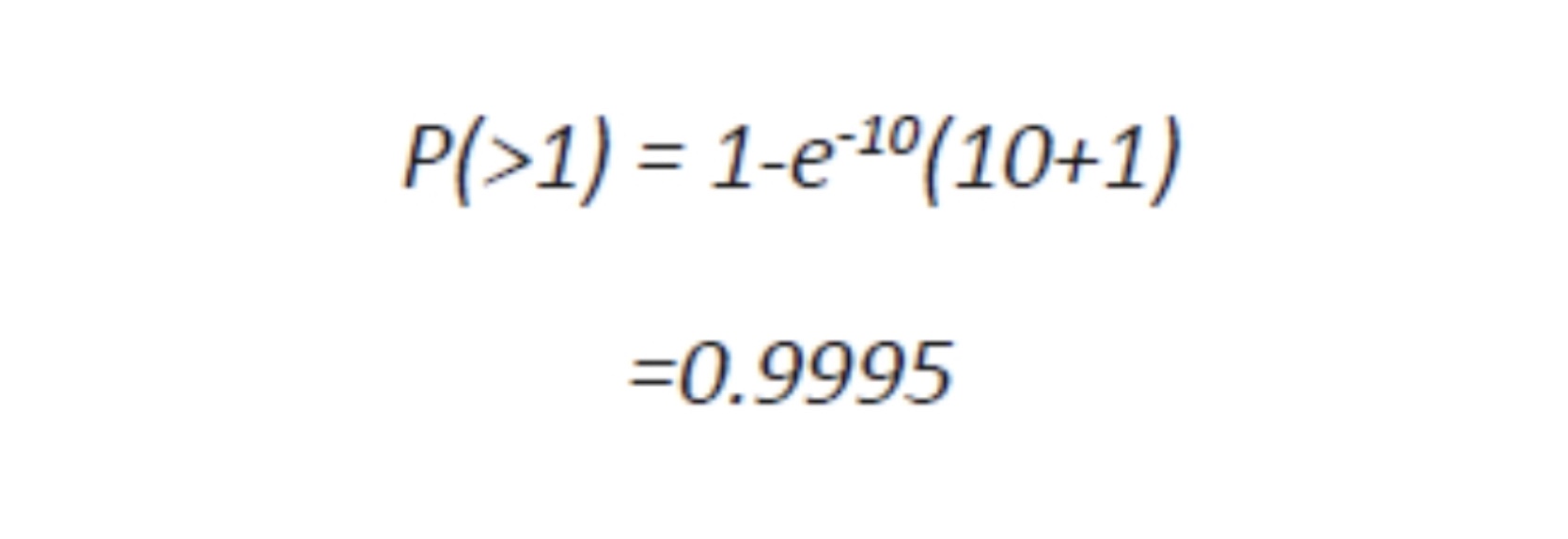
In many cultures of viruses, in order to infect most of the cells a MOI of 10 is used because for a million of target cells, less than a hundred should remain uninfected, a trivial number. In fact, in a culture of one million cells, 999,500 cells receive more than one virion:
In other words, it takes a certain number of microbes to cause an infection, or an obvious apparent infection such as illness or death. For instance, the infectious agent of Q Fever, the most infectious agent in the world, requires a single organism to cause disease, and for comparison, anthrax requires about 10,000 spores to kill a human. However, they are not uniformly applied to susceptible populations and many other factors control and confound their outbreaks as detectable disease. Although it is difficult to test this simple model in an uncontrolled population like humans or animals in the wild, it can and has been demonstrated and predictive in at least one case that supports the validity of the model: the eradication of smallpox in 1977. This global experiment was based on the assumption that If the proportion of the population that is immune exceeds the “herd immunity” for the infectious disease, then the disease can no longer be sustained in that population. In the case of smallpox, this level was exceeded by vaccination and the disease was consequently eliminated. It is hoped that this can be done with other diseases by vaccination such as with polio or by isolation and depopulation in the case of animals as with brucellosis in cattle in the United States or as rabies was in the United Kingdom. The reverse has been demonstrated by refusal to vaccinate children or by inadequate immunization because of changes in the vaccine or virulence of the pathogen, as in the cases of measles and whooping cough, respectively. How would we write this in mathematical terms to determine the number of individuals which should be vaccinated to protect the population? We would use the following formula:
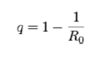
Where q equals the herd immunity, the portion of a population (or herd), which provides protection for individuals who have not developed immunity. As you can derive from the simple algebraic formula, the larger the reproduction number of the infectious disease the more the population has to be covered by vaccination.
A mathematical approach to increase the precision, accuracy and predictability of epidemiology, is the application of the “ROC curve” to determine if a disease can be “detected” in a population by infection and subsequent testing for that infection by some assay or observation of signs and symptoms. The “ROC curve”, Receiver Operating Characteristic was first used during World War II for the interpretation of radar signals before it was used in other types of sensors, including “sentinel” animals or humans who would indicate the presence of infectious diseases. Following the attack on Pearl Harbor in 1941, the United States Army began new research to increase the prediction of correctly detected Japanese aircraft from their radar signals, so was born the “ROC curve”. DARPA decided that the ROC curve would be the “gold standard” of detectability for biological agents. In the most general terms, the ROC curve is the fraction of true positives out of the total actual positives vs. the fraction of false positives out of the total actual negatives at various threshold settings. The ROC curve which applies to the ability of a sample to detect a positive for the presence of an infectious agent is an empirical plot of the number of infectious particles (bacteria or viruses) necessary to infect, or be “detected”, by the human or animal acting as a detector (actually measured by a clinical assay for the specific presence of the agent or the appearance of signs or symptoms which meets the case definition of the particular infectious disease) versus the false detection of such a particle. As the sensitivity of the detector is increased (equal to the number of true positives), the number of false positives increases sometimes linearly sometimes asymptotically or non-linearly depending on the characteristics of the detector. One has to decide the threshold of sensitivity vs acceptable false positives. The ROC curve is used to do this. The idea is to determine what you would expect for a given set of characteristics of the infection to be able to detect an infection. This approach tells the minimum number of samples from hosts, or the number of infected individuals in a given population that must be collected in the former and examined in the latter to detect an infection in a population, especially if it is not apparent or is endemic. In a sense, testing should tell the prevalence of the infection in the population in order to predict its Ro and growth rate of infection in that population, at least in theory. Bottom line is Ro is always being re-calculated from these data and testing results in addition to following numbers of cases over time (in realtime). It is more a result, an effect, an assessment, of where we stand in the fight against COVID and if we are approaching its end.